The Perceptron: A Probabilistic Model for Information Storage and Organization in the Brain
The first learning machine with a convergence guarantee: a linear threshold unit that adjusts its own weights from examples. It is the single neuron every deep network is built from — and the cautionary tale of what one neuron cannot do.
What · How · Why
What it is
The first machine that learns to classify patterns from examples rather than being hand-programmed — and the first with a proof that the learning will actually succeed when the two classes can be separated by a straight line. It is, quite literally, the single artificial neuron.
How it works
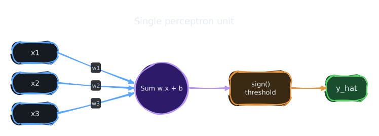
It computes a weighted sum of the inputs and fires "yes" if that sum clears a threshold. Training is dead simple: whenever it misclassifies an example, it nudges the weights a little toward the right answer. The convergence theorem proves this stops after at most \((R/\gamma)^2\) mistakes — a bound that depends only on the geometry of the data (its spread \(R\) and margin \(\gamma\)), not on the number of features.
Why it matters
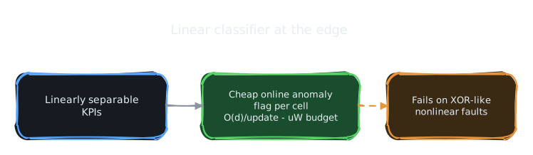
Every neuron in every deep network is a perceptron with a smooth activation, so this is the atom the whole field is built from. It is also the lightest possible learned classifier — ideal for ultra-constrained edge anomaly flags — but it can only draw straight boundaries, a limit that directly sets up Minsky & Papert and, eventually, the need for depth.
Round 1 — Core Claim & Mental Model
The problem it solves
Could a machine learn to classify patterns from data rather than being explicitly programmed? Rosenblatt's claim: a brain-inspired threshold unit can, by a simple error-correction rule, converge to weights that separate two classes — and provably so when the classes are linearly separable.
Mental model
A perceptron is a weighted voting booth. Each input feature casts a vote scaled by its weight; if the weighted sum clears a threshold, the unit fires "yes," else "no." Learning = nudging the weights toward voters who were right and away from voters who misled it, one mistake at a time.
Round 2 — Mathematical Model
The unit
\[ \hat{y} = \mathrm{sign}(w^{\top}x + b) \]The learning rule
On a misclassified example \((x,y)\) with \(y\in\{-1,+1\}\):
\[ w \leftarrow w + \eta\,y\,x,\qquad b \leftarrow b + \eta\,y \]Perceptron convergence theorem
If the data are linearly separable with margin \(\gamma\) and \(\|x\|\le R\), the number of updates is bounded:
\[ \#\text{mistakes} \;\le\; \left(\frac{R}{\gamma}\right)^2 \]Derivation sketch. Let \(w^*\) be a unit separator. Each update increases \(w^{\top}w^*\) by at least \(\eta\gamma\) (alignment grows linearly in updates \(k\)), while \(\|w\|^2\) grows by at most \(\eta^2R^2\) per step (norm grows like \(\sqrt{k}\)). Since \(\cos\angle(w,w^*)\le 1\), the linear-vs-\(\sqrt{k}\) race forces \(k\le (R/\gamma)^2\). The bound is independent of dimension — remarkable.
Complexity, invariants, limits
\(O(d)\) per update. Invariant: the bound depends only on geometry (\(R/\gamma\)), never on \(d\) or dataset size. Limiting case: as \(\gamma\to 0\) (classes touch) the bound diverges; for non-separable data the algorithm cycles forever — the defect Round 3 weaponizes.
How It Works & Visual Diagrams
Mathematical Proofs
The headline result is Novikoff's convergence theorem (1962): on linearly separable data the perceptron makes a finite, dimension-free number of mistakes. The proof is a two-sided squeeze — a linear lower bound and a square-root upper bound on the weight norm — closed by Cauchy–Schwarz.
- Lower bound on alignment. Project onto \(w^*\): \[ w_{k+1}^{\top}w^* = w_k^{\top}w^* + y\,(x^{\top}w^*) \ \ge\ w_k^{\top}w^* + \gamma, \] using the margin assumption. With \(w_0=0\), induction gives \(w_k^{\top}w^*\ \ge\ k\gamma.\)
- Upper bound on norm. Expand the squared norm: \[ \|w_{k+1}\|^2 = \|w_k\|^2 + 2\,y\,(w_k^{\top}x) + \|x\|^2 \ \le\ \|w_k\|^2 + \|x\|^2 \ \le\ \|w_k\|^2 + R^2, \] where the middle term is \(\le 0\) precisely because the update was a mistake. Induction gives \(\|w_k\|^2 \le kR^2.\)
- Squeeze (Cauchy–Schwarz). Since \(\|w^*\|=1\), \[ k\gamma \ \le\ w_k^{\top}w^* \ \le\ \|w_k\|\,\|w^*\| = \|w_k\| \ \le\ \sqrt{k}\,R. \] Dividing by \(\sqrt{k}\,\gamma\) yields \(\sqrt{k}\le R/\gamma\), i.e. \(k\le (R/\gamma)^2.\) ∎
Cross-links: the same margin quantity \(\gamma\) reappears as the SVM objective (maximize \(\gamma\)); the dimension-free flavour foreshadows generalization bounds. The “no nonlinear separator” defect is made precise in Minsky & Papert (1969), and repaired by backpropagation (1986).
Round 3 — Limitations & Community Response
Linear only. A single perceptron can represent only linearly separable functions. It famously cannot compute XOR. Convergence is guaranteed only under separability; otherwise it never halts and the weights oscillate.
The hype and the backlash. Rosenblatt and the press overclaimed ("machines that will walk, talk, see, write"). Minsky & Papert's 1969 book Perceptrons rigorously characterized these limits, and — fairly or not — is widely credited with redirecting funding away from connectionism for over a decade (the first "AI winter").
What it lacked. No method to train hidden layers; no nonlinearity that was differentiable. Both were resolved by backpropagation (1986), which is why this node points forward to it.
Round 4 — AI × Networks Connection
AI lineage. Every neuron in a modern deep net is a perceptron with a smooth activation; the dot-product-then-nonlinearity motif recurs in MLP blocks, including the feed-forward sublayers of the Transformer. Understanding the perceptron's geometry is the cleanest entry to decision boundaries.
Networks angle. Linear threshold classifiers remain the right tool when compute is brutally scarce: per-cell anomaly flags, admission-control heuristics, and lightweight RAN policies where an \(O(d)\) update must run inside a tight power/latency envelope. The perceptron defines the floor of the ML-for-RAN design space.
Verify — Credibility Check
The convergence theorem is a proved mathematical result (Novikoff 1962 gave the clean margin-bound proof) and is reproduced in every learning-theory course; it is not in dispute. The contemporaneous empirical/engineering claims about the Mark I Perceptron hardware were overstated relative to what a single layer can do — the math is solid, the marketing was not. Single test that bounds its power: present XOR; a one-layer perceptron provably cannot fit it, which is exactly the falsification Minsky & Papert formalized.
- For edge RAN, where does the cost/benefit line sit between an \(O(d)\) linear flag and a small nonlinear model — is there a margin \(\gamma\) below which only the latter is worth the power?
- Can the margin bound \((R/\gamma)^2\) give a useful a-priori estimate of how many labeled fault examples an online edge classifier needs before it stabilizes?
- How much of a Transformer's power is "just" stacked perceptrons vs the attention mixing — i.e. what does the MLP-only ablation lose?