Language Models are Few-Shot Learners

papers Brown et al. (OpenAI) · 2020 Round 4 ✓ math ✓ visual ✓

GPT-3: a 175-billion-parameter Transformer that performs new tasks from a few examples in its prompt — no gradient updates. It demonstrated that scale alone produces in-context learning, reframing "training a model per task" into "prompting one general model."

What · How · Why

What it is

GPT-3 is a 175-billion-parameter Transformer that performs brand-new tasks from just a few examples written into its prompt — with no retraining, no gradient updates. It demonstrated that sheer scale, on its own, produces a general-purpose capability called in-context learning.

How it works

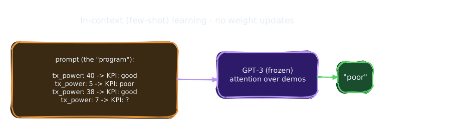
It is trained on one humble objective — predict the next token — over a huge slice of the internet. At inference, you put a few worked examples in the prompt; the frozen model reads them with attention, infers "what task is this?", and continues the pattern. The reason this is worth billions: test loss falls as a smooth power law in model size, data, and compute (scaling laws), so capability is predictable as you scale up. Think of the prompt as the program and the weights as a fixed interpreter.

Why it matters

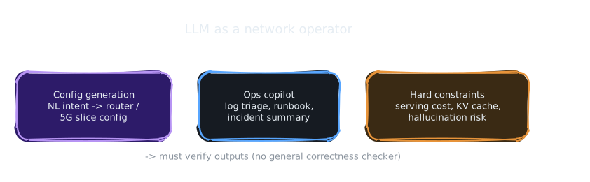
It turned "train a separate model per task" into "prompt one general model," launching the LLM industry and the prompt-engineering era. For AI × Networks it is the engine of LLM-based network config generation and ops copilots — but deployment runs straight into the Attention paper's O(n²)/KV-cache serving costs and the Turing/Rice reality that no general checker can verify generated configs, so outputs must be validated against a restricted, decidable policy.

Round 1 — Core Claim & Mental Model

The problem it solves

Pre-2020 NLP needed task-specific fine-tuning datasets for every task. The claim: a sufficiently large autoregressive LM, trained only to predict the next token, acquires a general skill — in-context learning — letting it do translation, QA, arithmetic, or code from a handful of prompt examples, weights frozen.

Mental model

The prompt is the program; the weights are the interpreter. Instead of editing the interpreter (fine-tuning), you specify the task by demonstration inside the input. The model infers "what task am I doing?" from the pattern of examples and continues it. Scale is the active ingredient: the capability emerges as parameters and data grow.

Spatial metaphor: meta-learning by reading. During pretraining the model implicitly learns many tasks; at inference, a few examples select which of those latent skills to apply — like recognizing a genre from its first paragraph and writing in it.

Round 2 — Mathematical Model

Training objective

Plain autoregressive maximum likelihood — minimize next-token cross-entropy (Shannon's source coding again):

\[ \mathcal{L} = -\sum_{t} \log P_\theta(x_t \mid x_{In-context learning, formally

For a $k$-shot task, condition on a context of demonstrations and predict:

\[ P_\theta\big(y \mid \underbrace{(x_1,y_1),\dots,(x_k,y_k)}_{\text{demonstrations}},\, x_{\text{query}}\big) \]

No parameter update occurs; "learning" happens in the forward pass via attention over the demonstrations.

Scaling laws (the theoretical backbone)

Test loss falls as a power law in parameters $N$, data $D$, and compute $C$ (Kaplan et al. 2020):

\[ L(N) \approx \left(\frac{N_c}{N}\right)^{\alpha_N},\qquad \alpha_N \approx 0.076 \]

Smooth, predictable improvement over orders of magnitude — the empirical license for spending $millions on one training run.

Scale & complexity

175B parameters, 96 layers, $d_{\text{model}}=12288$, 96 heads, context 2048 tokens; trained on ~300B tokens. Compute $\sim 3.14\times10^{23}$ FLOPs. Inference cost $\approx 2N$ FLOPs/token (≈350 GFLOPs/token) plus the Transformer's $O(n^2)$ attention over context — the source of serving cost and the KV-cache memory problem.

Invariants & limiting cases

Few-shot ≥ one-shot ≥ zero-shot, and the gap widens with model size — larger models are better in-context learners. Limiting cases: $k=0$ (zero-shot) relies purely on pretraining priors; very long contexts hit the quadratic-attention wall; below a parameter threshold, in-context learning barely appears (an emergence phenomenon).

How It Works & Visual Diagrams

In-context learning — Architecture: the task is specified by demonstrations in the prompt; the frozen model infers the pattern via attention and completes the query. The "learning" is a forward pass.

GPT-3 for networks — Intersection diagram: few-shot prompting enables LLM-based network config generation and ops copilots — gated by serving cost, KV-cache memory, and the need to verify outputs (Turing/Rice: no general correctness checker).

Mathematical Proofs

GPT-3's training objective rests on two exact facts — the autoregressive factorization and the entropy lower bound on cross-entropy — plus one empirical regularity (scaling laws) whose compute-optimal allocation we derive exactly given its functional form. The paper is candid that scaling is measured, not proven; we keep that line sharp.

Proposition 1 — The autoregressive factorization is exact For any sequence distribution, $\displaystyle P(x_{1:T})=\prod_{t=1}^{T}P(x_t\mid x_{<t}).$ Minimizing the next-token cross-entropy therefore fits the full joint, not an approximation of it.

Proof. Repeatedly apply the definition of conditional probability (the chain rule): $P(x_1,x_2)=P(x_1)P(x_2\mid x_1)$, and inductively $P(x_{1:t})=P(x_{1:t-1})P(x_t\mid x_{<t})$. Telescoping from $t=1$ to $T$ gives the product. The training loss $\mathcal L=-\sum_t\log P_\theta(x_t\mid x_{<t})$ is exactly $-\log P_\theta(x_{1:T})$, so minimizing it is maximum-likelihood on the joint. ∎

Proposition 2 — Cross-entropy ≥ entropy (Gibbs' inequality) For the true next-token distribution $p$ and model $q$, \[ H(p,q)=-\sum_{x}p(x)\log q(x)\ \ge\ H(p)=-\sum_x p(x)\log p(x), \] with equality iff $q=p$. The loss is floored by the entropy (rate) of language itself.

Proof. The gap is the Kullback–Leibler divergence: $H(p,q)-H(p)=\sum_x p(x)\log\frac{p(x)}{q(x)}=D_{\mathrm{KL}}(p\,\|\,q)$. By Jensen's inequality applied to the concave $\log$, \[ -D_{\mathrm{KL}}(p\,\|\,q)=\sum_x p(x)\log\frac{q(x)}{p(x)}\ \le\ \log\sum_x p(x)\frac{q(x)}{p(x)}=\log\sum_x q(x)=\log 1=0, \] so $D_{\mathrm{KL}}\ge0$, i.e. $H(p,q)\ge H(p)$; equality holds iff $q=p$ almost everywhere (strict concavity of $\log$). Thus a perfect language model converges to the entropy rate of text — the direct heir of Shannon's source-coding bound, now as a learning target. ∎

Proposition 3 — Compute-optimal allocation under a scaling law The scaling law $L(N)\approx (N_c/N)^{\alpha_N}$ is an empirical power-law fit (not a theorem). But given a separable loss $L(N,D)=A\,N^{-\alpha}+B\,D^{-\beta}+L_\infty$ and compute budget $C\approx 6ND$, the optimal split is fixed: \[ N^\star\propto C^{\,\beta/(\alpha+\beta)},\qquad D^\star\propto C^{\,\alpha/(\alpha+\beta)}. \]

Proof. Minimize $L$ subject to $6ND=C$. Form the Lagrangian $\mathcal L=A N^{-\alpha}+B D^{-\beta}+L_\infty-\lambda(6ND-C)$. Stationarity: \[ -\alpha A N^{-\alpha-1}=6\lambda D,\qquad -\beta B D^{-\beta-1}=6\lambda N. \] Dividing the two equations eliminates $\lambda$: $\dfrac{\alpha A N^{-\alpha-1}}{\beta B D^{-\beta-1}}=\dfrac{D}{N}$, i.e. $\alpha A\,N^{-\alpha}=\beta B\,D^{-\beta}$ — the two loss terms scale together. Substituting the constraint $D=C/6N$ gives $N^\star\propto C^{\beta/(\alpha+\beta)}$ and hence $D^\star\propto C^{\alpha/(\alpha+\beta)}$. GPT-3 sat at large $N$, small $D$; the same algebra with the measured exponents later (Chinchilla, 2022) showed the optimum wanted far more data — a correction to, not a refutation of, the power law. ∎

Interpretation 4 — In-context learning as implicit inference With demonstrations $(x_i,y_i)$ in the prompt, the model's prediction can be read as marginalizing a latent task $\theta$: \[ P\big(y\mid x,\text{prompt}\big)=\int P(y\mid x,\theta)\,P\big(\theta\mid \text{prompt}\big)\,d\theta. \]

Status — interpretation, not theorem. This is the Bayesian account of in-context learning (Xie et al., 2021): pretraining on documents with latent structure makes the conditional $P(\theta\mid\text{prompt})$ concentrate on the demonstrated task, so no weights change — “learning” is posterior updating in the activations. It is a model of the phenomenon supported by synthetic experiments, not a proof about GPT-3's internals; the paper reports the behavior empirically and leaves the mechanism open. ∎

Cross-links: the entropy floor ties training to Shannon (1948); the inability to verify generated programs/configs is Turing/Rice undecidability; the architecture being scaled is the Transformer. Scaling laws remain empirical — the open question is whether they have a derivable origin.

Round 3 — Limitations & Community Response

Brittle, ungrounded, expensive. Few-shot performance is sensitive to prompt wording and example order; the model hallucinates, struggles with multi-step arithmetic/reasoning, and has no grounding in truth. At 175B params it is costly to serve and its 2048-token context is small by later standards.

What came after. The paper undersold reasoning (later unlocked by chain-of-thought prompting) and omitted alignment — InstructGPT/RLHF (2022) showed instruction tuning + human feedback matters as much as raw scale. Chinchilla (2022) then corrected the compute-optimal balance: GPT-3 was under-trained on data for its size; smaller models on more tokens do better. So GPT-3's specific scaling choices were superseded even as its thesis held.

Reception & risks. Enormously influential — it launched the prompt-engineering era and the LLM industry. The paper itself foregrounds risks: bias, misinformation, energy/carbon cost, and data contamination of benchmarks (test data leaking into the web-scraped training set), which complicates clean evaluation.

Round 4 — AI × Networks Connection

AI lineage (capstone). GPT-3 is the Transformer (2017) scaled until a new behavior — in-context learning — emerged, trained by backprop (1986) on the cross-entropy objective whose optimality Shannon (1948) established, all running on the Universal Machine (Turing, 1936). It is where the whole lineage in this KB converges.

Networks angle (direct intersection backlog item). Few-shot prompting is the engine of LLM for network configuration generation: natural-language intent → device/slice config, plus ops copilots for log triage and runbooks. But deployment collides with the serving cost and KV-cache memory limits from the Attention node, and with a Turing/Rice reality — there is no general verifier of generated-config correctness, so outputs must be validated against a restricted, decidable policy fragment before use.

→ Attention 2017 (the architecture) → Turing 1936 (no general verifier) → AI×Net: LLM network config generation

Verify — Credibility Check

Architecture facts (confirmed): 175B parameters, 96 layers, $d_{\text{model}}=12288$, 96 attention heads, 2048-token context, ~300B training tokens. Plausibility of results: most benchmarks are externally reproducible (the API was widely tested), and the scaling-law backbone has been independently re-derived. Two honest caveats the authors themselves raise: (1) benchmark contamination — web-scraped training data may overlap test sets, inflating some scores; (2) few-shot numbers vary with prompt design, so single-point claims are noisy. The cleanest replication/falsification is the scaling-law prediction: train models across sizes and check the power-law fit — which Chinchilla did, confirming the trend while revising the optimal $N$:$D$ ratio.

Open questions this raises:

Can LLM-generated network configs be constrained to a provably-decidable policy DSL so outputs are verifiable (closing the Turing/Rice gap), without losing the few-shot convenience?
What is the smallest model (post-Chinchilla, data-optimal) that retains reliable in-context learning for RAN config tasks, given edge serving and KV-cache budgets?
Does in-context learning over network telemetry beat a fine-tuned small model on cost-adjusted accuracy — i.e., when is prompting the right tool vs a dedicated traffic model?